RNN and LSTM
nn.embedding
nn.embedding 构造一个vocab size的lookup table,每个vocabulary用hidden_size维度的向量表示
>>> embedding = nn.Embedding(10, 3)
>>> embedding.weight

# Parameter containing:
# tensor([[ 1.2402, -1.0914, -0.5382],
#         [-1.1031, -1.2430, -0.2571],
#         [ 1.6682, -0.8926, 1.4263],
#         [ 0.8971, 1.4592, 0.6712],
#         [-1.1625, -0.1598, 0.4034],
#         [-0.2902, -0.0323, -2.2259],
#         [ 0.8332, -0.2452, -1.1508],
#         [ 0.3786, 1.7752, -0.0591],
#         [-1.8527, -2.5141, -0.4990],
#         [-0.6188, 0.5902, -0.0860]], requires_grad=True)

>>> embedding.weight.size
# torch.Size([10, 3])
# note that input is indices, the size of which is [2,4]
input = torch.LongTensor([[1,2,4,5],[4,3,2,9]])

a = embedding(input)
print(a)
# tensor([[[-1.1031, -1.2430, -0.2571],
#          [ 1.6682, -0.8926, 1.4263],
#          [-1.1625, -0.1598, 0.4034],
#          [-0.2902, -0.0323, -2.2259]],
#         [[-1.1625, -0.1598, 0.4034],
#          [ 0.8971, 1.4592, 0.6712],
#          [ 1.6682, -0.8926, 1.4263],
#          [-0.6188, 0.5902, -0.0860]]], grad_fn=<EmbeddingBackward>)

print(a.size())
# torch.Size([2, 4, 3])
a = embedding(input)是去embedding.weight中取对应index的词向量!
看a的第一行,input处index=1,对应取出weight中index=1的值,即按index取词向量!
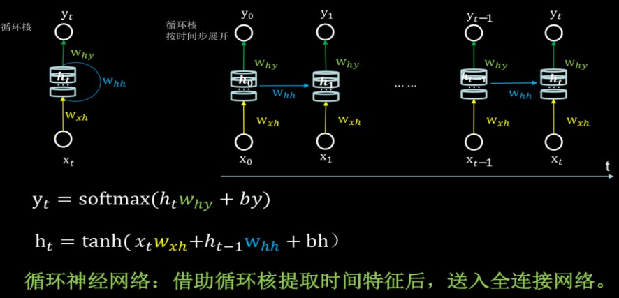
Vanilla RNN
bs = 20
vocab_size =10000

class three_layer_recurrent_net(nn.Module):
	def __init__(self, hidden_size):
        super(three_layer_recurrent_net, self).__init__()
			self.layer1 = nn.Embedding( vocab_size  , hidden_size )
			self.layer2 = nn.RNN(       hidden_size , hidden_size )
			self.layer3 = nn.Linear(    hidden_size , vocab_size  )

        def forward(self, word_seq, h_init ):
			g_seq = self.layer1( word_seq )
			h_seq , h_final  =  self.layer2( g_seq , h_init )
			score_seq = self.layer3( h_seq )
return score_seq, h_finalnn.RNN(input_size, hidden_size, num_layers=1, nonlinearity=tanh, bias=True, batch_first=False, dropout=0, bidirectional=False)
input_size输入特征的维度, 一般rnn中输入的是词向量,那么 input_size 就等于一个词向量的维度(nn.Embedding()里定义了词向量维度),或词向量的feature。
hidden_size隐藏层神经元个数,或者也叫输出的维度(因为rnn输出为各个时间步上的隐藏状态),可以不等于input_size,网络中会自动进行升降维度。
num_layers: Number of recurrent layers. Setting num_layers=2 would mean stacking two RNNs together to form a stacked RNN, with the second RNN taking in outputs of the first RNN and computing the final results. Default: 1
nonlinearity激活函数,只能用relu或tanh(默认)
bias是否使用偏置
batch_first输入数据的形式
dropout是否在每个recurrent layer(RNN layer)后应用dropout(除最后一层),默认不使用,如若使用将其设置成一个0-1的数字即可
birdirectional是否使用双向的 rnn,默认是 False,双向RNN对输入输出维度会有影响
# 输入
input_shape为[seq_length, batch_size, hidden_size]
在例子里,g_seq是size为[word_seq, hidden_size]的张量,或者可以写成[seq_length, batch_size, hidden_size]
h_init的shape为[num_layers, batch_size, hidden_size]
# 输出
在前向计算后会分别返回输出output和隐藏状态h_n。其中输出指的是隐藏层在各个时间步上计算并输出的隐藏状态,它们通常作为后续输出层的输⼊。需要强调的是,该“输出”本身并不涉及输出层计算,size为[seq_length, batch_size, hidden_size];隐藏状态指的是隐藏层在最后时间步的隐藏状态:当隐藏层有多层时,每⼀层的隐藏状态都会记录在该变量中,隐藏状态h的size为[num_layers, batch_size, hidden_size]

input_size = 5(word vector dimension or input feature), hidden_size = 6, num_layers = 2
rnn = nn.RNN(5, 6, 7)

input = torch.randn(21, 8, 5)

# seq_length = 21, (21 words, 21 time_steps), batch_size = 8, (8 sentences), every single word vector’s size = 5
# 假设一个batch里面有8个句子,现在走到第17个time step,同时计算的是这个batch里面,8个不同sequence中第17个词,得到这8个词的状态之后,传到下一个timestep对应的cell,再计算8个不同sequence中第18个词
# num_layer = 7, batch_size = 8, hidden_size = 6

h0 = torch.randn(7, 8, 6)
output, hn = rnn(input, h0)

# output.size() = torch.Size([21, 8, 6])
# hn.size() = torch.Size([7, 8, 6])
Why tanh?
RNN的每个时间步的权重是相同的,bp过程相当于权重的连续相乘,因此比CNN更容易出现梯度消失和梯度爆炸,因此采用tanh比较多。tanh也会出现梯度消失和梯度爆炸,但是相比于Sigmoid[0, 0.25]更好
RNN training in 10 epoch
hidden_size=150
net = three_layer_recurrent_net( hidden_size )
criterion = nn.CrossEntropyLoss()
my_lr = 1
seq_length = 35
start=time.time()
for epoch in range(10):
	# keep the learning rate to 1 during the first 4 epochs, then divide by 1.1 at every epoch
	if epoch >= 4:
		my_lr = my_lr / 1.1
	# create a new optimizer and give the current learning rate.
	optimizer=torch.optim.SGD( net.parameters() , lr=my_lr )
	# set the running quantities to zero at the beginning of the epoch
    running_loss=0
    num_batches=0
    # set the initial h to be the zero vector
    h = torch.zeros(1, bs, hidden_size)
    # send it to the gpu
    h=h.to(device)

	for count in range( 0 , 46478-seq_length ,  seq_length):
        # Set the gradients to zeros
        optimizer.zero_grad()
        # create a minibatch, every unit output should be compared with the next step,
        # so minibatch_label should be [ count+1 : count+seq_length+1 ]
        minibatch_data = train_data[  count  :  count+seq_length  ]
        minibatch_label = train_data[ count+1 : count+seq_length+1 ]
        # send them to the gpu
        minibatch_data=minibatch_data.to(device)
        minibatch_label=minibatch_label.to(device)
        # Detach to prevent from backpropagating all the way to the beginning
        # Then tell Pytorch to start tracking all operations that will be done on h
        h=h.detach()
        h=h.requires_grad_()
        # forward the minibatch through the net
        scores, h = net( minibatch_data, h )
        # reshape the scores and labels to huge batch of size bs*seq_length
        scores = scores.view( bs*seq_length , vocab_size)
        minibatch_label =  minibatch_label.view( bs*seq_length )
        # Compute the average of the losses of the data points in this huge batch
        loss = criterion( scores , minibatch_label )
        # backward pass to compute dL/dR, dL/dV and dL/dW
        loss.backward()
        # do one step of stochastic gradient descent: R=R-lr(dL/dR), V=V-lr(dL/dV), ...
        utils.normalize_gradient(net)
        optimizer.step()
        # update the running loss
        running_loss += loss.item()
        num_batches += 1

	# compute stats for the full training set
	total_loss = running_loss/num_batches
	elapsed = time.time()-start
	print('')
	print('epoch=',epoch, '\t time=', elapsed,'\t lr=', my_lr, '\t exp(loss)=', math.exp(total_loss))
	eval_on_test_set()
LSTM
help alleviate the problem of vanishing and exploding gradients in RNN
长短期记忆(LSTM),隐藏状态是⼀个元组(h, c),即hidden state和cell state
其中的input
input(seq_len, batch_size, input_size)seq_len:在文本处理中,如果一个句子有7个单词,则seq_len=7;在时间序列预测中,假设我们用前24个小时的负荷来预测下一时刻负荷,则seq_len=24。
batch_size:一次性输入LSTM中的样本个数。在文本处理中,可以一次性输入很多个句子;在时间序列预测中,也可以一次性输入很多条数据。
input_size:在文本处理中,由于一个单词没法参与运算,因此我们得通过Word2Vec来对单词进行嵌入表示,将每一个单词表示成一个向量,此时input_size=embedding_size。比如每个句子中有五个单词,每个单词用一个100维向量来表示,那么这里input_size=100;在时间序列预测中,比如需要预测负荷,每一个负荷都是一个单独的值,都可以直接参与运算,因此并不需要将每一个负荷表示成一个向量,此时input_size=1。 但如果我们使用多变量进行预测,比如我们利用前24小时每一时刻的[负荷、风速、温度、压强、湿度、天气、节假日信息]来预测下一时刻的负荷,那么此时input_size=7
class three_layer_recurrent_net(nn.Module):
	def __init__(self, hidden_size):
		super(three_layer_recurrent_net, self).__init__()
			self.layer1 = nn.Embedding( vocab_size , hidden_size )
			self.layer2 = nn.LSTM(   hidden_size , hidden_size )
			self.layer3 = nn.Linear(  hidden_size , vocab_size  )
		def forward(self, word_seq, h_init, c_init ):
			g_seq = self.layer1(word_seq )
			h_seq,(h_final,c_final) = self.layer2( g_seq , (h_init,c_init) )
			score_seq = self.layer3(h_seq)
			return score_seq, h_final , c_final

lstm = nn.LSTM(10, 20, 2)
input = torch.randn(5, 3, 10)
h0 = torch.randn(2, 3, 20)
c0 = torch.randn(2, 3, 20)
output, (hn, cn) = lstm(input, (h0, c0))